Tutorial: Illumination Correction

Prospective correction uses additional images obtained at the time of image capture. Two types of additional images can be used:

• A dark image is an image of the scene background acquired with no light.
• A bright image is an image of the scene background acquired with light but without objects.

dark = ∑ darki
bright = ∑ brighti

1. Correction from a Dark Image and a Bright Image

The corrected image g(x,y) is obtained using the following transformation:

            f(x,y) - d(x,y)
   g(x,y) = --------------- .C
            b(x,y) - d(x,y)

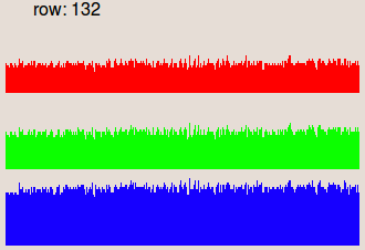
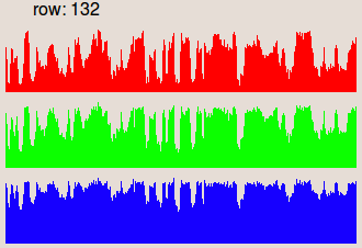
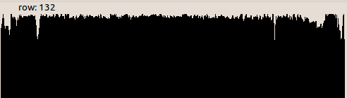
where f(x,y) is the original image, d(x,y) is the dark image, b(x,y) is the bright image, and C is a normalization constant used to recover the original colors:

                                  1
    C = mean(f(x,y)) . ----------------------
                           f(x,y) - d(x,y) 
                     mean( --------------- )
                           b(x,y) - d(x,y)  

where mean(i(x,y)) is the mean value of the image i(x,y).

Pandore Script (bash)

psub serous.pan dark.pan tmp1.pan
psub bright.pan dark.pan tmp2.pan
pdiv tmp1.pan tmp2.pan tmp3.pan
pmeanvalue tmp3.pan c1.pan
pdivval c1.pan tmp3.pan tmp4.pan
pmeanvalue serous.pan c2.pan
pmultval c2.pan tmp4.pan output.pan

Results

The images in the second row are the profiles of the row 132, where the gray level values are represented as vertical bars. We notice that in the input image the illumination is higher on the right side than on the left side. This is corrected in the result image.

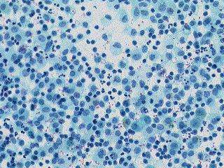Input image.	Dark image.	Bright image.	Corrected output image.
Profile of the row 132.	Profile of the row 132.	Profile of the row 132.	Profile of the row 132.

2. Correction from a Bright Image

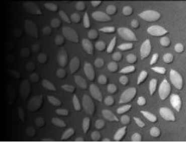
If only the bright image is available, the method uses division of the source image by the bright image if the image acquisition device is linear, or the subtraction of the source image with the bright if the acquisition device is logarithmic with a gamma of 1.

In case of a linear acquisition device, the corrected image g(x,y) is obtained using the following transformation:

            f(x,y)
   g(x,y) = ------ . C
            b(x,y)

where f(x,y) is the original image, b(x,y) is the bright image, and C is a normalization constant that is used to recover the initial colors:

                           1
   C = mean(f(x,y)) . ------------
                           f(x,y)
                     mean( ------ )
                           b(x,y)

where mean(i(x,y)) is the mean value of the image i(x,y).

Pandore Script (bash)

pdiv grain.pan grain_background.pan tmp1.pan
pmeanvalue grain.pan c1.col
pmultval c1.col tmp1.pan tmp2.pan
pmeanvalue tmp1.pan c2.col
pdivval c2.col tmp2.pan grain_out.pan

Results

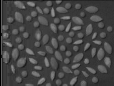Input image.	Background image.	Output image.
Profile of the row 132.	Profile of the row 132.	Profile of the row 132.

3. Correction from a Dark Image

If only the dark image is available, the method consists in subtraction of the dark image with the original image. The corrected image g(x,y) is then obtained using the following transformation:

   g(x,y) = f(x,y) - d(x,y) + mean(d(x,y))

where f(x,y) is the original image, d(x,y) is the dark image and mean(d(x,y)) is the mean value of the dark image.

Pandore Script (bash)

psub serous.pan dark.pan tmp1.pan
pmeanvalue dark.pan c.col
paddval c.col tmp1.pan out.pan

Results

Input image.	Dark image.	Output image.
Profile of the row 132.	Profile of the row 132.	Profile of the row 132.

II. Retrospective correction

When additional image are not available, an ideal illumination model has to be estimated to define the bright image. Therefore, retrospective correction can use the same background subtraction method than the prospective correction with the estimated bright image.

There are different algorithms for estimating the bright image. All of them assume the scene background corresponds to the low frequencies and the objects to the high frequencies. The retrospective correction techniques consist in removing the objects from the background to build the bright image, and then apply the same techniques as the prospective correction.

1. Retrospective Correction using Low-pass Filtering

The background is estimated by using a low-pass filtering with a very large kernel. The background is then subtracted from the input image to compensate the illumination.
The corrected image g(x,y) is obtained from the input image f(x,y) by:

   g(x,y) = f(x,y) - LPF(f(x,y)) + mean(LPF(f(x,y)))

where LPF(f(x,y)) is the low-pass filtering of image f(x,y), and mean(LPF(f(x,y))) is the mean value of the low pass image.

The following example uses the Gaussian filter with a kernel of size 20, greater than the size of the characters.

Pandore Script (bash)

pgaussianfiltering 20 page.pan mask.pan
psub page.pan mask.pan tmp.pan
pmeanvalue mask.pan c.col
paddval c.col tmp.pan out.pan

Results

Input image.	Estimated background image.	Output image.
Profile of the row 132.	Profile of the row 132.	Profile of the row 132.

2. Retrospective Correction using Homomorphic Filtering

The background is estimated by using homomorphic filtering with a low-pass filter. Homomorphic principle is to remove high frequencies (considered as reflectance) and keep the low frequencies (considered as illumination). The background is removed by highpass filtering the logarithm of the image and then taking the exponent (inverse logarithm) to restore the image.

The corrected image g(x,y) is obtained from the input image f(x,y) by:

   g(x,y) = exp(LPF(log(f(x,y)))) . C

where LPF(f(x,y)) is the low-pass filter of f(x,y) and C is the normalization coefficient given by:

              mean(f(x,y))
   C = ----------------------------
                  f(x,y)
       mean( --------------------- )
              exp(LPF(log(f(x,y))))

where mean(i(x,y)) is the mean value of the image i(x,y).

The following example uses the Butterworth filter with a cutoff value of 3.

Note that this technique does not really yield accurate results.

Pandore Script (bash)

cutin=0
# the less the cutoff value, the stronger filtering.
cutoff=3
order=2

homomorphicfiltering(){
    paddcst 1 $1 i0.pan # The zero log problem
    plog i0.pan i0.pan
    psetcst 0 i0.pan i1.pan
    pfft i0.pan i1.pan i2.pan i3.pan
    pproperty 0 i2.pan
    ncol2=`pstatus`
    pproperty 1 i2.pan
    nrow2=`pstatus`
    pproperty 2 i2.pan
    ndep2=`pstatus`
    pbutterworthfilter $ncol2 $nrow2 $ndep2 0 $cutin $cutoff $order i4.pan 
    pmult i2.pan i4.pan i5.pan
    pmult i3.pan i4.pan i6.pan
    pifft i5.pan i6.pan i7.pan i8.pan
    
    pproperty 0 $1
    ncol1=`pstatus`
    pproperty 1 $1
    nrow1=`pstatus`
    pproperty 2 $1
    ndep1=`pstatus`

    pextractsubimage 0 0 0 $ncol1 $nrow1 $ndep1 i7.pan i9.pan
    pexp i9.pan i11.pan
    paddcst -1 i11.pan i12.pan
    
    pclipvalues 0 255 i12.pan  i13.pan
    pim2uc i13.pan $2
}
    
multiplicative-correction() {
    pdiv $1 $2 i14.pan
    pmeanvalue $1 col.pan; c1=`pstatus`
    pmeanvalue i14.pan col.pan; c2=`pstatus`
    c=`echo "scale = 1; $c1/$c2" | bc`
    
    pmultcst $c i14.pan $3
}

pproperty 3 page.pan; bands=`pstatus`
if [ $bands -eq 1 ]
then
    # grayscale image
    homomorphicfiltering page.pan mask2.pan
    multiplicative-correction page.pan mask2.pan out.pan
else
    # color image
    pimc2img 0 input1.pan r.pan
    pimc2img 1 input1.pan g.pan
    pimc2img 2 input1.pan b.pan
    homomorphicfiltering r.pan maskr.pan
    homomorphicfiltering g.pan maskg.pan
    homomorphicfiltering b.pan maskb.pan
    multiplicative-correction r.pan maskr.pan outr.pan
    multiplicative-correction g.pan maskg.pan outg.pan
    multiplicative-correction b.pan maskb.pan outb.pan 
    pimg2imc 0 outr.pan outg.pan outb.pan out.pan
fi

Results

Input image.	Estimated background image.	Output image.
Profile of the row 132.	Profile of the row 132.	Profile of the row 132.

3. Retrospective Correction using Morphological Filtering

The background is estimated by mathematical morphology opening or closing. The estimated background is then subtracted from the original image. The total sequence of operations corresponds to a top hat of the image. Top hat removes high frequencies (considered as reflectance) and keeps low frequencies (considered as illumination). Black top hat is used for clear background and white top hat is used for dark background.

If the background is clear, the corrected image g(x,y) is obtained using:

   g(x,y) = BTH[f(x,y)] + mean(closing(f(x,y)))
   g(x,y) = [f(x,y) - closing(f(x,y))] + mean(closing(f(x,y)))

where mean(closing(f(x,y))) is the mean value of the closed image.

The following example uses a disc structuring element with size 11, greater than the size of the objects (characters).

Pandore Script (bash)

# black top hat
pdilatation 2 5 page.pan b.pan
perosion 2 5 b.pan mask3.pan
psub page.pan mask3.pan tmp.pan
# normalization
pmeanvalue mask3.pan c.col
paddval c.col tmp.pan out.pan

Results

Input image.	Estimated background image.	Output image.
Profile of the row 132.	Profile of the row 132.	Profile of the row 132.

4. Retrospective Correction using Linear Regression

The background is estimated by using orthogonal linear regression. The background is approximated by a plane, so it is not suitable for complex background.

The corrected image g(x,y) is obtained from the input image f(x,y) by:

   g(x,y) = (f(x,y) - LR(f(x,y)) - mean(LR(f(x,y)))

where LR(f(x,y)) is the linear regression of f(x,y) in x and y, and mean(LR(f(x,y))) is the mean value of the linear regression image.

Pandore Script (bash)

plinearregression page.pan mask4.pan
psub page.pan mask4.pan tmp.pan
pmeanvalue mask4.pan c.col
paddval c.col tmp.pan out.pan

Results

Input image.	Estimated background image.	Output image.
Profile of the row 132.	Profile of the row 132.	Profile of the row 132.

5. Retrospective Correction Based on Surface Fitting with polynomial

The background is estimated from a least square fitting of a polynomial that approximates the background. The background is then subtracted from the input image to compensate the illumination. The corrected image g(x,y) is obtained from the input image f(x,y) by:

   g(x,y) = (f(x,y) - b(f(x,y))) - mean(b(f(x,y)))

where b(f(x,y)) is a polynomial that approximates the background, and mean(b(f(x,y))) is the mean value of the polynomial image.

In the following examples, two types of polynomials has been used:

• Second-order polynomial
• Legendre polynomial.

Second-Order Polynomial

The first following example uses second-order polynomial. The operator needs a mask to select only background pixels. The mask defines the list of pixels that can be used to compute the polynomial approximation.

The order of the polynomial can be selected separately for x, y, and mixed terms. For example, with orders 2, 3, and 2 for x, y, and xy respectively, the polynomial will be:

  a+b*x+c*x^2+d*y+e*y^2+f*y^3+g*xy

Pandore Script (bash)

ppolynomialfitting 2 2 1 page.pan page_mask.pan mask5.pan
psub page.pan mask5.pan tmp.pan
pmeanvalue mask5.pan c.col
paddval c.col tmp.pan out.pan

Results

Input image.	Mask image.	Estimated background image.	Output image.
	.
Profile of the row 132.	.	Profile of the row 132.	Profile of the row 132.

Legendre Polynomial

The second following example uses Legendre polynomial. This technique uses the orthogonality relation of the Legendre polynomials to expand an image as a double sum of those functions. The sum is then evaluated to produce an image that approximates a projection onto the space of polynomial images.

Pandore Script (bash)

plegendrepolynomialfitting 2 2 page.pan mask6.pan
psub page.pan mask6.pan tmp.pan
pmeanvalue mask6.pan c.col
paddval c.col tmp.pan out.pan

Results

Input image.	Estimated background image.	Output image.
Profile of the row 132.	Profile of the row 132.	Profile of the row 132.

6. Retrospective Correction for Color Images

The previous methods cannot be applied per se to color images because they used channel-wise processing and thus alter the spectral composition of colors (creation of new colors).

The solution is to convert the image into the HSL color space and applied the correction to the lightness channel.