 IMAGE Team - The Pantheon project
Rescaling or resampling is the technique used to create a new version of an image with a different size. Increasing the size of the image is called upsampling, and reducing the size of an image is called downsampling.
It turns out that these operations are not lossless. For example, if you downsample an image and then upsample the resulted image, you will get a sightly different image than the original. This is a non trivial process that involves a trade-off between efficiency, smoothness, sharpness and speed. That's why there exist different algorithms.Pandore supports several different algorithms to perform resampling. Each of them have their own advantages and drawbacks in terms of lossless, blur, and speed.
We present here a list of examples that use the Pandore operators to realize the resampling. We distinguish the case of image downsampling and image upsampling because the algorithms can have different performance in each case.
Image upsampling is illustrated with the small image below which is magnified by 400% (x4).

 |
 |
| Nearest Neighbor Resampling | Bilinear Resampling |
|---|---|
prescale 4 4 0 jellybeans.pan result.pan |
plinearrescale 4 4 0 jellybeans.pan result.pan |
 |
 |
| Hermite Resampling | Bell Resampling |
phermiterescale 4 4 0 jellybeans.pan result.pan |
pbellrescale 4 4 0 jellybeans.pan result.pan |
 |
 |
| Mitchell Resampling | Bicubic Resampling |
pmitchellrescale 4 4 0 jellybeans.pan result.pan |
pbicubicrescale 4 4 0 jellybeans.pan result.pan |
 |
|
| Lanczos Resampling | |
planczosrescale 4 4 0 jellybeans.pan result.pan |
Image upsampling is illustrated with the small image below which is magnified by 400% (x 4).

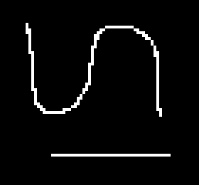 |
 |
| Nearest Neighbor Resamplingn | Bilinear Resampling |
|---|---|
prescale 4 4 0 binarysmall.pan result.pan |
plinearrescale 4 4 0 binarysmall.pan result.pan |
 |
 |
| Hermite Resampling | Bell Resampling |
phermiterescale 4 4 0 binarysmall.pan result.pan |
pbellrescale 4 4 0 binarysmall.pan result.pan |
 |
 |
| Mitchell Resampling | Bicubic Resampling |
pmitchellrescale 4 4 0 binarysmall.pan result.pan |
pbicubicrescale 4 4 0 binarysmall.pan result.pan |
 |
|
| Lanczos Resampling | |
planczosrescale 4 4 0 binarysmall.pan result.pan |
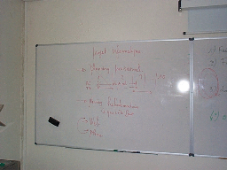
Image downsampling is illustrated with the image below which is reduced by 400% (x 0.4).
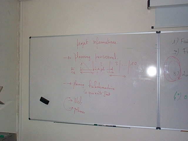
 |
 |
| Nearest Neighbor Resampling | Bilinear Resampling |
|---|---|
prescale 0.4 0.4 0 whiteboard.pan result.pan |
plinearrescale 0.4 0.4 0 whiteboard.pan result.pan |
 |
 |
| Hermite Resampling | Bell Resampling |
phermiterescale 0.4 0.4 0 whiteboard.pan result.pan |
pbellrescale 0.4 0.4 0 whiteboard.pan result.pan |
 |
 |
| Mitchell Resampling | Bicubic Resampling |
pmitchellrescale 0.4 0.4 0 whiteboard.pan result.pan |
pbicubicrescale 0.4 0.4 0 whiteboard.pan result.pan |
 |
|
| Lanczos Resampling | |
planczosrescale 0.4 0.4 0 whiteboard.pan result.pan |
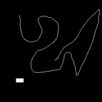
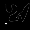
The various algorithms are applied to the binary image below which is reduced by 400% (x0.4).
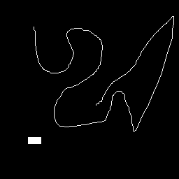
 |
 |
| Nearest Neighbor Resampling | Bilinear Resampling |
|---|---|
prescale 0.4 0.4 0 binary.pan result.pan |
plinearrescale 0.4 0.4 0 binary.pan result.pan |
 |
 |
| Hermite Resampling | Bell Resampling |
phermiterescale 0.4 0.4 0 binary.pan result.pan |
pbellrescale 0.4 0.4 0 binary.pan result.pan |
 |
 |
| Mitchell Resampling | Bicubic Resampling |
pmitchellrescale 0.4 0.4 0 binary.pan result.pan |
pbicubicrescale 0.4 0.4 0 binary.pan result.pan |
 |
|
| Lanczos Resampling | |
planczosrescale 0.4 0.4 0 binary.pan result.pan |
When an image is scaled up to a larger size, there is a question of what will be the color of the new pixels in between the original pixels. When an image is scaled down to a lower size, the inverse question is what will be the color of the remaining pixels. There exists several answers to these questions.
To simplify the presentation, consider the case of an 1D image f(x) that we want to magnify by a factor of 2 to create the new image g(x). Mathematically, this is formulated as:
g(x) = f(x/2)
Consider a concrete example for f(x) with the sample values [2, 3, 5, 4, 3, 2, 4]. This provides the image here-after (where the image is represented by its profile, the gray levels are visualized in height):
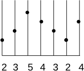
We want to double the size of the image f(x) to create the image g(x)
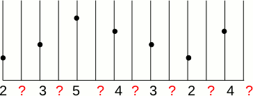
Therefore, we have to determine what will be the value of the new pixels.
There are two obvious answers:
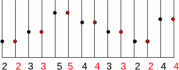
If we want to triple the size of the image f(x) then the resulted image g(x) is:

To reduce the image size by a factor of n, the inverse principle of the nearest neighbor is to choose 1 pixel out of n.
The second answer consists in using the weighted average value of the nearest known pixels according to their distance to the unknown pixel. The easiest way to visualize this, is to draw a line between two consecutive unknown pixels and to pick the value along the line for the unknown pixels. This solution is called "linear interpolation" since it use straight lines between samples.
The result is the image g(x) :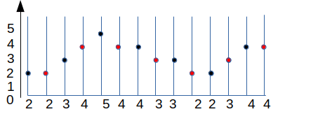
To reduce the image size by a factor of n, the new value of the mean value of the n nearest pixels.
One may wonder which of the previous method is "best". The answer is "it depends". In case of intensity image, the second solution is the best one because the first produces blocky effects whilst the second produces a smoother image. However, in case of region maps, the first solution is the only possible solution since the first one add new labels.
Before considering the 2D, we examine a less intuitive but more general way to implement these methods: convolution. The convolution defines a general principle for the interpolation. The interpolation kernel k(i) defines the list of neighbors to be considered and the weight assigned to them for calculating the value of the central pixel. Mathematically, this corresponds to the operation:

By choosing the suitable filter, we can define different types of reconstruction. For example, the nearest neighbor interpolation with left priority to double the size is implemented by the convolution kernel [1, 1, 0]. Linear interpolation can be implemented by the kernel [0.5 1 0.5]. For other distances, we just use other kernels. For example, the nearest neighbor kernel for size tripling is [0, 1, 1, 1, 0] and the linear interpolation kernel is [1/3, 2/3, 1, 2/3, 1 / 3].
To illustrate the principle of interpolation with a convolution kernel, consider the case of the bilinear kernel for size doubling. The first is to double the size of f(x). Then the new pixels is set to 0 to produce the image f'(x). From there, convolution is applied to produce g(x). Thus, the value at the coordinate 6 is: 1*34+0*2/3+0*1/3+0*2/3+0*1/3.

The value at the coordinate 7 is: 39 = 1/3*50 + 2/3*34.

This implementation by convolution has several advantages:
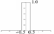
Within the convolution framework, it is easy to vary the types of kernel and thus the type of interpolation. As we saw earlier, the simplest kernel is the nearest neighbor kernel, which corresponds to a box. It produces images with blocky effect.

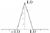
Linear interpolation use a convolution kernel k(x) which has the shape of a triangle. The output image thus has a smoother surface because the discretization is less strong.

But the transition betwen two pixels can be smoother if curve is used instead of straight line.

In general, B-splines are used to model the transition between two original pixels. The B-spline curves are described by a series of polynomials with a given degree. The higher the degree, the higher the variations in the curve.
A B-spline of degree 1 is formed by a series of straight lines, and therefore corresponds to a bilinear kernel. A B-spline of degree 2 is composed of a series of parabolic curves and B-spline of degree 3 is composed of cubic curves.
The previous description done for 1D can easily be extended to 2D and 3D. The only difference is that convolution is performed along the x, y and z axis. For example the following formulae is used for 2D interpolation:

The different kernels developed in Pandore for 2D and 3D images are described in the following sections.
The color of a pixel in the result image is the color of the nearest pixel of the original image. If we enlarge an image by 2, one pixel will be enlarged to 2x2 area with the same color. If we shrink an image by 2, only 1 pixel over 2x2 pixels is retained in the output image. The interpolation kernel k(x) is simply:
   k(x) = | 1 ; if |x| < 0.5
          | 0 ; otherwise
|
|
This operator produces blocky effects on result in case of upsampling and removes thin edges in case of downsampling. However, it is the fastest algorithm and it is the only one that does not insert new colors in the result.
Bilinear sampling considers the closest 2x2 neighborhood of known pixel values surrounding the unknown pixel. It can be implemented by the triangle kernel k(x):
   k(x) = | 1-|x| ; |x| < 1
          | 0 ; sinon
|
|
Bell resampling uses a convolution kernel to interpolate the pixels of the input image in order to calculate the pixel values of the output image. The Bell convolution kernel k(x) is defined as:
          | 0.75-|x|2 ; if |x| < 0.5
   k(x) = | 0.5 * (|x|-1.5)2 ; if 0.5 < |x| <1.5
          | 0 ; otherwise
|
Hermite resampling uses a convolution kernel to interpolate the pixels of the input image in order to calculate the pixel values of the output image. Hermite is a particular case of the bicubic algorithm, where a=0. The Hermite convolution kernel k(x) is defined as:
   k(x) = | 2|x|3 - 3|x|2 + 1 ; if |x| ≤ 1
          | 0 ; otherwise
|
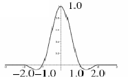
For bicubic resampling, the convolution kernel is composed of piecewise cubic polynomials. The output pixel value is a weighted sum of pixels in the nearest 4-by-4 neighborhood. The kernel is k(x):
          | (a+2)|x|3 - (a+3)|x|2+1 ; if x ≤ 1
   k(x) = | a|x|3 - 5a|x|2 +8a|x| - 4a ; if 1 < x < 2
          | 0 ; otherwise
where a=-0.5 in the present implementation. Note that if a=0, the algorithm is equivalent to the Hermite algorithm. |
|
It is probably the most used of the resampling algorithm in image manipulation software programs.
Mitchell resampling uses a convolution kernel to interpolate the pixels of the input image in order to calculate the pixel values of the output image. It is also a bicubic filter.
The Mitchell convolution kernel k(x) is defined as:
where B=1/3, and C=1/3.
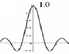
Lanczos resampling uses a convolution kernel
to interpolate the pixels of the input image in order to calculate the
pixel values of the output image. The Lanczos convolution kernel k(x)
is defined as:III.10. Lanczos Resampling
|
This algorithm provides the best results, however it is extremely time-consuming.